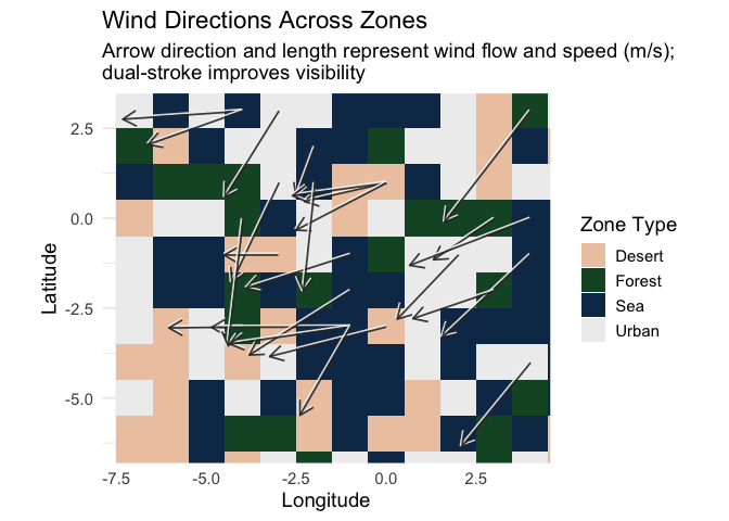
ggtwotone extends ggplot2 with dual-stroke and contrast-aware geoms that improve the visibility of annotations, curves, and labels on heterogeneous backgrounds. The package is designed for figures containing images, maps, heatmaps, microscopy data, or other complex visualizations where standard single-color annotations may become difficult to distinguish.

Documentation

Complete documentation, reference manuals, and additional examples are available at Reference Manual, or see them in the R help tab after loading the package.

Key Features

Dual-stroke segments
Dual-stroke curves and paths
Dual-stroke regression lines
Contrast-aware text labels
Automatic highlight palettes
WCAG/APCA-based color utilities

Why ggtwotone?

Standard annotations often become difficult to distinguish on complex or heterogeneous backgrounds, such as microscopy images, maps, photographs, or heatmaps. ggtwotone addresses this problem by combining dual-stroke rendering with contrast-aware color selection.

Improved visibility
Better accessibility
Grayscale-friendly figures
Publication-ready graphics

Installation

Development version

# install.packages("pak")
pak::pak("bwanniarachchige2/ggtwotone")

(After CRAN release this section will simply become install.packages("ggtwotone").)

Quick Example

The example below demonstrates how geom_segment_dual() and geom_text_contrast() improve measurement overlays on a microscopy image.

library(ggtwotone)
library(magick)

img_path   <- "man/figures/micro_image.jpg"
um_per_px  <- 0.05                  # <-- calibration: micrometers per pixel
bar_um     <- 10                    # scale bar length in micrometers

# Load image as a background grob
img <- magick::image_read(img_path)
w   <- magick::image_info(img)$width
h   <- magick::image_info(img)$height
bg  <- grid::rasterGrob(img, width = unit(1, "npc"), height = unit(1, "npc"))


meas <- data.frame(
  x = 0.3218, y = 0.4507, xend = 0.7974, yend = 0.6371   # <-- adjust to your line
)

# Compute physical length for the label
dx_px  <- abs(meas$xend - meas$x) * w
dy_px  <- abs(meas$yend - meas$y) * h
len_um <- sqrt(dx_px^2 + dy_px^2) * um_per_px
lab    <- sprintf("%.1f \u00B5m", len_um)

# Midpoint for the label
xm <- (meas$x + meas$xend)/2
ym <- (meas$y + meas$yend)/2
lab_df <- data.frame(x = xm, y = ym + 0.05, label = lab)

#Plot
ggplot() +
  # background SEM image
  annotation_custom(bg, xmin = 0, xmax = 1, ymin = 0, ymax = 1) +
  # measurement line with dual stroke
  geom_segment_dual(
    data = meas,
    aes(x = x, y = y, xend = xend, yend = yend),
    colour1 = "#0D0D0D",
    colour2 = "#FFFFFF",
    linewidth = 1.2,
    lineend = "round",
    arrow = grid::arrow(ends = "both", length = unit(0.18, "in"), type = "open") 
  ) +
  # measurement label (contrast-aware)
  geom_text_contrast(
    data = lab_df,
    aes(x = x, y = y, label = label),
     background = "#444444",
    size = 4.2
  ) +
  coord_fixed(xlim = c(0, 1), ylim = c(0, 1), expand = FALSE) +
  theme_void()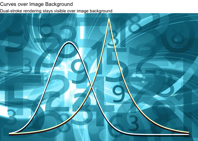

Dual-stroke annotations remain clearly visible regardless of the local background, while labels automatically adapt to maintain contrast.

Image credit

SEM micrograph adapted from Marie Majaura, Own work, licensed under CC BY-SA 3.0. Used under the terms of the license.

Additional Example

The following example demonstrates geom_text_contrast() on a confusion matrix generated from a linear discriminant analysis (LDA) classifier fitted to the iris data. Text colours are selected automatically to maintain readability against tiles with different background colours.

library(dplyr)
library(ggplot2)
library(ggtwotone)
library(scales)
library(MASS)

set.seed(1)

# Fit LDA classifier on iris
iris_lda <- MASS::lda(
  Species ~ Sepal.Length + Sepal.Width + Petal.Length + Petal.Width,
  data = iris
)

iris_pred <- predict(iris_lda)$class

# Build confusion matrix
classes <- levels(iris$Species)

cm <- table(
  True = iris$Species,
  Predicted = iris_pred
) |>
  as.data.frame()

cm <- cm |>
  group_by(True) |>
  mutate(
    Accuracy = Freq / sum(Freq),
    label = sprintf("%.1f%%", 100 * Accuracy)
  )

# Palette and background colors for text contrast
pal <- c("#313695", "#74add1", "#fdae61", "#fee08b")

col_fun <- scales::col_numeric(
  palette = pal,
  domain = c(0, 1)
)

cm$fill_hex <- col_fun(cm$Accuracy)

# Plot
ggplot(cm, aes(Predicted, True)) +
  geom_tile(aes(fill = Accuracy), color = "white", linewidth = 0.8) +
  geom_text_contrast(
    aes(label = label),
    background = cm$fill_hex,
    base_colour = "#004488",
    method = "auto",
    contrast = 4.5,
    size = 5,
    fontface = "bold"
  ) +
  scale_fill_gradientn(
    colours = pal,
    limits = c(0, 1),
    name = "Accuracy"
  ) +
  coord_fixed() +
  labs(
    title = "Confusion Matrix for Iris LDA",
    x = "Predicted Species",
    y = "True Species"
  ) +
  theme_minimal(base_size = 13) +
  theme(
    panel.grid = element_blank(),
    axis.text.x = element_text(angle = 45, hjust = 1)
  )

geom_text_contrast() automatically selects a readable foreground color for each label based on the tile background, improving readability while preserving the underlying color scale.

Citation

If you use ggtwotone in published work, please cite

citation("ggtwotone")

(after the package is available on CRAN).

License

MIT License.